Trouble that you can't fix: omitted variable bias

 

credit: SkipsterUK (CC BY-NC-ND 2.0)

Preamble

In the previous post in this series, I explained how to use causal diagrams to set up multivariate regressions so that statistical confounding is eliminated.

In this post, I'll give a short and simple example of a case where statistical confounding can't be prevented, because an important variable is unavailable. This sort of thing is unfixable, and it is bound to happen sometimes in observational statistical analyses, because there are influencing variables that we just don't anticipate, and therefore don't collect.

Here's the entire 'statistical confounding' series:

• Part 1: Statistical confounding: why it matters
  

  - on the many ways that confounding affects statistical analyses.
  

• Part 2: Simpson's Paradox: extreme statistical confounding 

  - understanding how statistical confounding can cause you to draw exactly the wrong conclusion.

• Part 3: Linear regression is trickier than you think 

  - a discussion of multivariate linear regression models

• Part 4: A gentle introduction to causal diagrams 

  - a causal analysis of fake data relating COVID-19 incidence to wearing protective glasses.

• Part 5: How to eliminate confounding in multivariate regression 

  - how to do a causal analysis to eliminate confounding in your regression analyses

• Part 6: A simple example of omitted variable bias (this post) 

  - an example of statistical confounding that can't be fixed, using only 4 variables.

How to eliminate confounding in multivariate regression

 

Great grey owl (Creative Commons).

Preamble

For my previous post on causal diagrams, I made up a fake dataset relating the incidence of COVID-19 to the wearing of protective goggles for hypothetical individuals. The dataset included several related covariates, such as whether the person in question was worried about COVID-19. 

The goal of the exercise was to (hypothetically!) determine whether protective glasses was an effective intervention for COVID-19, and to see how accidental associations due to other variables could mess up the analysis.

I faked the data so that COVID-19 incidence was independent of whether the person wore protective goggles. But then I demonstrated, using multivariate regressions, that it is easy to incorrectly conclude that protective glasses are significantly effective for reducing the risk of COVID-19. I also showed how a causal diagram relating the variables can be used to determine which variables to include and exclude from the analysis.

In this article, I'll explain how to recognize the patterns in causal diagrams that lead to statistical confounding, and show how to do a causal analysis yourself.

Here's the entire 'statistical confounding' series:

- Part 1: Statistical confounding: why it matters: on the many ways that confounding affects statistical analyses 

- Part 2: Simpson's Paradox: extreme statistical confounding: understanding how statistical confounding can cause you to draw exactly the wrong conclusion

- Part 3: Linear regression is trickier than you think: a discussion of multivariate linear regression models

- Part 4: A gentle introduction to causal diagrams: a causal analysis of fake data relating COVID-19 incidence to wearing protective goggles

- Part 5: How to eliminate confounding in multivariate regression (this post): how to do a causal analysis to eliminate confounding in your regression analyses    

-Part 6: A simple example of omitted variable bias: an example of statistical confounding that can't be fixed, using only 4 variables.

Introduction

In A gentle introduction to causal diagrams, I introduced a fake dataset in which rows represented individuals, containing the following information:

- $C$: does the person test positive for COVID-19?
- $G$: does the person wear protective glasses in public?
- $W$: is the person worried about COVID-19?
- $S$: does the person avoid social contact?
- $V$: is the person vaccinated?


I then did some multivariate logistic regressions to answer the following question: does wearing protective goggles help reduce the likelihood of catching COVID-19?

In generating the dataset, I made the following assumptions:

- protective glasses have no direct effect on COVID-19 incidence;
- avoiding social contact has a significant negative effect on COVID-19 incidence;
- getting vaccinated has a very significant negative effect on COVID-19 incidence;
- being worried about COVID makes a person much more likely to get vaccinated, avoid social contact, and wear protective glasses;
- being vaccinated makes a person less likely to avoid social contact. 

The causal diagram associated with these variables and assumptions is shown below. An arrow from one variable to another indicates that the value of the 'to' variable depends on the 'from' variable. 

The exercise in the article was to determine which variables to include in a multivariate regression, in order to analyze whether protective glasses reduce the risk of catching COVID-19. The colored nodes are the ones that were ultimately included; only the $W$ (worried about COVID-19) variable was used as a covariate, in addition to the dependent and independent variables $G$ and $C$. 

 

Backdoor paths

In the diagram above, the causal relationship we want to assess (between $G$ and $C$) is represented by the gray dashed arrow. But there are a lot of other connections with intermediate variables, in the form of paths in the graph between $G$ and $C$, that can accidentally generate statistical associations between $G$ and $C$.

The first such path is shown below: it passes from $G$ to $W$ to $S$ to $C$. This is called a 'backdoor path' because arrow 1 points into $G$, rather than emitting from $G$. This path can be described in words as follows: if the person is worried about COVID-19, this makes her more likely to both wear protective glasses and socially distance. Since social distancing is an effective intervention against COVID-19, this sets up a negative correlation between wearing glasses and catching COVID-19; but the dataset was constructed so that protective glasses had no impact on COVID-19, so the effect is only due to correlation, not causation.

A second path is shown below: it passes from $G$ through $W$ to $V$ and then to $C$. In words: If a person is worried about COVID-19, he is more likely to both wear protective glasses and to get vaccinated. Since vaccination is an effective intervention against COVID-19, this again sets up a negative correlation between wearing glasses and catching COVID-19.

A third path is shown below: it passes from $G$ through $W$ to $V$, then to $S$ and finally $C$. In words: if a person is worried about COVID-19, she is more likely to get vaccinated, after which she may be less likely to socially distance. This is a problem in our analysis if we do not know the person's vaccination status, since the presence of a lot of people who do not socially distance, and yet do not catch COVID-19, will obscure the effectiveness of social distancing as an intervention. In the presence of enough vaccine-positive people, it might even appear that people who do not socially distance are *less* likely to get COVID-19 if we don't know people's vaccination status!

There is another type of backdoor path to consider, shown below. Backdoor path 4 passes from $G$ to $W$, through $S$ and $V$, to $C$. Backdoor path 4 will not cause confounding unless we make the mistake of conditioning on variable $S$.  The variable $S$ is called a collider variable, because it has two arrows in the path pointing into it. We have to be careful not to condition on a collider variable, i.e., not to include it in the multivariable regression.

Patterns of confounding

Each of the backdoor paths in any causal diagram can be broken down into a series of connections among three variables in the path. There are 3 relationships that can occur among these 3 variables: the 'fork' pattern, the 'pipe' pattern, and the 'collider' pattern.
 

Fork pattern

The image below shows the 'fork' pattern, which occurs in our example among the variables $G, W$, and $S$. The fork occurs when a single variable affects two 'child' variables; in this case, being worried makes a person both more likely to socially distance, and more likely to wear protective glasses.

If three variables are related by the fork pattern, then the two child variables will be marginally statistically dependent, but will be independent if we condition on the parent variable. Mathematically, the fork pattern says that:

$$p(G, W, S) = p(G|W)p(S|W)p(W).$$

Since $p(G,S)=\int p(G|V)p(S|V)p(V) dV$, it follows that $p(G,S)\ne p(G)\cdot p(S)$ in general. However, $p(G,S|V)=p(G|V)\cdot p(S|V)$; in this graph of 3 variables, $W$ and $S$ are conditionally independent given $V$.

In words, this says that if I know whether a person is worried about COVID-19, then knowing whether a person socially distances tells me nothing additional about whether they are likely to wear glasses.

Pipe pattern

The image below shows the 'pipe' pattern, which occurs in our example among the variables $W, S$, and $C$. The pipe occurs when a variable is causally 'in-between' two other variables. In this case, being worried causes a person to socially distance, which in turn reduces their chance of getting COVID-19. 

If three variables are related by the pipe pattern, then the two outer variables will be marginally statistically dependent, but will be independent if we condition on the inner variable. Mathematically, $p(W,C)\ne p(W)\cdot p(C)$ in general, but $p(W,C|S)=p(W|S)p(C|S)$. The fork and pipe patterns are alike in this regard.

In words, this says that if I know whether a person is avoiding social contact, then knowing whether the person is worried about COVID-19 tells me nothing additional about whether they might have caught it.

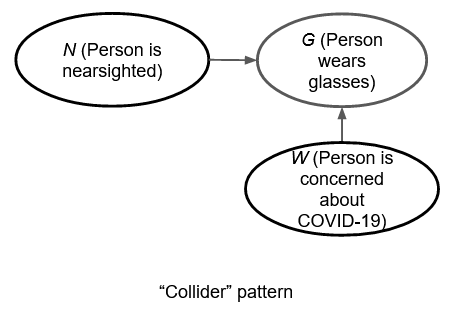
Collider pattern

The collider pattern occurs when a single variable is dependent on two unrelated parent variables. There aren't any simple collider pattern examples in our example causal diagram -- for example, social distancing $S$ is dependent both on $V$ and $W$, but these two variables are also directly related to each other. So I've added an extra random variable in the diagram below: $N$, which is 1 if the person is nearsighted, and 0 otherwise. Clearly, being nearsighted is another reason why someone might wear glasses. 

The collider pattern is different from the fork and pipe patterns. In the collider pattern, the two parents of the common child are marginally independent of each other. Mathematically, we have $p(N,W) = p(N)p(W)$ (it follows from the definition of the joint distribution, $p(N,W,G)=p(G|N,W)p(N)p(W)$), but $p(N,W|G)\ne p(N|G)\cdot p(W|G)$ in general. In other words, conditioning the regression on the 'collider variable' $G$ causes the parent variables $N,W$ to become associated. But the association is purely statistical; the two parent variables are still causally unrelated.

To see why this happens, imagine that you know nothing about whether a person wears glasses or not. Then knowing in addition that the person is nearsighted gives you no additional information about whether they are worried about COVID-19.

But suppose that you now know that the person is wearing glasses (i.e., you are conditioning on $G=1$). If you know in addition that the person is not nearsighted, then the odds are higher that they are wearing glasses because they are worried about COVID-19; and if you know that they are not worried about COVID-19, the odds increase that they are wearing glasses because they are nearsighted. So the parent variables become related. Collider bias is sometimes called 'explaining away'; knowing that a person is nearsighted 'explains away' their reason for wearing glasses.  
 

Putting it together

This tells you everything you need to know in order to construct an unconfounded multivariate regression analysis, in order to determine whether one variable has a causal impact on another. The game is to 'block all the backdoor paths', to prevent them from causing accidental correlations between the dependent and independent variables.

For example, consider 'backdoor path 1' at the beginning of the article. This path contains a fork pattern (the variable $W$, pointing to $G$ and $S$) and a pipe pattern (the variable $S$, which is pointed to by $W$, and which points to $C$). If we don't condition on $W$ or $S$, then these variables will set up associations between $G$ and $S$, and between $W$ and $C$; the unbroken line of associations sets up a relationship between $G$ and $C$ that is only a correlation, not causal.

In order to prevent this from happening, we need to condition on either $W$ or $S$. We must choose one of them; conditioning on either one of them will break that chain of association. This is called 'blocking the backdoor path'. But blocking one backdoor path isn't enough; we must block all of them.

Consider backdoor path 2 from $G$ to $C$; it contains a fork variable, $W$, and a pipe variable, $V$. Conditioning on either $V$ or $W$ will block backdoor path 2. Note that conditioning on $W$ will block both backdoor paths 1 and 2, but conditioning on $V$ or $S$ will leave one of the paths unblocked.

Now consider backdoor path 3. Backdoor path 3 contains a fork variable, $W$; a pipe variable, $V$; and another pipe variable, $S$. Conditioning on any of these will block this backdoor path, so again, $W$ will work for this path.

Finally, looking at backdoor path 4, we see that $S$ is a collider variable in this path. Looking at this path in isolation, $W$ and $V$ will be marginally independent of each other. But if we condition on the variable $S$, that will set up an association between $W$ and $V$, which will connect all the variables in backdoor path 4, and cause confounding.

The following shows how the association between $W$ and $V$ can occur, as a result of knowing the value of $S$. Suppose we know for sure that a person is not avoiding social contact (i.e., we have conditioned on $S$). Suppose we also know that this person is worried about COVID-19; then this makes it highly likely that the person is vaccinated, since they would otherwise be avoiding people. Conversely, if we know that a person is not avoiding social contact, and we also know that the person is not vaccinated, then it is highly likely that they just aren't worried about COVID-19.   

The fact that $S$ is a collider in this path means that we have to avoid conditioning on $S$ (including it in the regression). Conditioning on it will open backdoor path 4, which would otherwise be blocked.  

To summarize, there are 5 total backdoor paths in this diagram -- the four we have discussed, and one other that also contains the variable $S$ as a collider (see if you can find it). Conditioning on $W$ will block the first 3 backdoor paths, and will not accidentally unblock the two paths that contain $S$ as a collider variable. Therefore, a multivariate regression that contains only $W$ as a covariate, $G$ as the independent variable, and $C$ as the dependent variable, will correctly show that wearing glasses has no effect on COVID-19 incidence.

 

A gentle introduction to causal diagrams

 

Cute burrowing owl. (creative commons)

 In a recent blog post, Statistical confounding: why it matters, I touched a bit on the topic of causal diagrams, and defined statistical confounding as occurring when the association between two variables is influenced by a third variable, leading (potentially) to incorrect conclusions about the causal relationship between them. 

In this blog post, I'll work through an example of a simple (and totally hypothetical! but nevertheless kind of plausible!) causal diagram, and show how it can be used to select variables for multiple regressions so that causality can be inferred. Please note that this is a completely made-up example using data that I generated. I've just made up a story around COVID-19 because it is an important statistical problem to which most people can intensely relate!

Imagine that we've collected data for a huge observational study, in an attempt to determine whether wearing protective glasses affects the likelihood of catching COVID-19. Our dataset consists of many thousands of rows of data; each row represents an individual. The dataset has two columns: $G$, a boolean variable indicating whether the person wears protective glasses, and $C$, a boolean variable indicating whether the person has tested positive for covid. The causal relationship we want to test can be diagrammed like this:

 

 where an arrow from $G$ to $C$ indicates that glasses-wearing has a causal effect on catching COVID-19. 

I've generated some data representing the results of such an observational study. Because I faked the data, I know for certain that there is no direct causal impact of $G$ on $C$ in it; $C$ is generated from an expression that doesn't include $G$.  The generated data includes $G$ and $C$ and several other boolean variables, including $W$ (is the person concerned about COVID-19?) and $S$ (is the person avoiding social contact?).

The diagram below shows the true causal relationships among these 4 random variables. There is no directed arrow between $G$ and $C$, indicating that wearing protective glasses neither prevents nor causes a person to catch COVID-19. There are arrows from $W$ to both $G$ and $S$, indicating that concern about COVID-19 drives people to both wear protective glasses, and to socially distance. There is an arrow from $S$ to $C$, indicating that avoiding social contact actually does prevent catching COVID-19.

 But let's suppose we don't know anything about the data. In order to investigate the question of whether glasses-wearing helps prevent COVID-19, we do a Bayesian logistic regression using the following model:

$$
\begin{aligned}  
C_i &\sim\text{Bernoulli}(p) \\  
\text{logit}(p) &= \alpha_0 + \alpha_{[G_i]}\\
\alpha_0 & \sim N(\mu=0, \sigma=1.5) \\
\alpha_{[G_i]} & \sim N(\mu=0, \sigma=3)  
\end{aligned}  
$$

where $G_i$ is either 0 or 1. The line $\text{logit}(p)=\alpha_0+\alpha_{[G_i]}$ indicates that we are modeling the probability of catching COVID-19 as a function only of $G$ (wearing protective glasses); we aren't including any other covariates.

We fit this model, and find that the differences between the values of the model's posterior parameters $\alpha_{[G==0]}$ and $\alpha_{[G==1]}$ are large, indicating that protective glasses make a difference. The graph below shows the histogram of the differences between the fitted values of $\alpha_{[G==0]}$ and $\alpha_{[G==1]}$; more than 95% of the histogram's mass lies between the red lines, to the right of 0.

In fact, the mean fitted (posterior) probability of catching COVID-19 is 0.02 for the group that does not wear protective glasses, and 0.005 for the group that does wear protective glasses. Can we conclude that wearing protective glasses reduces the risk of catching covid by a factor of about 4?

Well, no. But this set of causal relationships can nevertheless produce values of $G$ and $C$ that make it look like wearing protective glasses is highly effective for preventing COVID-19. This is because we've messed up by using a model that depends only on $G$ and $C$.

In the diagram below, the causal relationship we want to assess is represented by the gray arrow between $G$ and $C$ (these are in red, indicating that they were included in the regression model). But there is a second path in the graph from $G$ to $C$ that can generate an association between $G$ and $C$, the one from $G$ to $W$ to $S$ to $C$. Unlike the one we want to test, it is a 'back-door' path from $G$ to $C$, meaning that it starts with a causal arrow that points *into* $G$ rather than away from $G$.

Here's what's going on: the factor $W$ is driving both glasses-wearing $G$ (an ineffective intervention) and social distancing $S$ (the effective intervention). This creates an association between $G$ and $S$: if a person is wearing protective glasses, they are highly likely to also be social distancing, and vice-versa. Therefore, a person wearing protective glasses is probably also social distancing, and therefore is less likely to catch COVID-19. And so, if all you're using in your model are the variables $G$ and $C$, it looks like wearing protective glasses is effective against COVID-19.

But if you then pass a law that everyone has to wear protective glasses, it will have no effect on the COVID-19 rate, and you'll have spent a lot of political capital getting an ineffective resolution passed, and people won't listen to your advice anymore. This is a bad outcome.  

How can we fix this statistical problem?

If the above causal diagram is the true one (a big if!), then we can fix it. We need to have collected not only the values of $G$ and $C$, but also those of $S$. What we are going to do is to 'block the back-door path' from $G$ to $C$ by conditioning on $S$, which (in the regression context) means we are going to include $S$ as a variable in the regression model. We write the new model as:

$$
\begin{aligned}  
C_i &\sim\text{Bernoulli}(p) \\  
\text{logit}(p) &= \alpha_0+\alpha_{[G_i]} +\alpha_{[S_i]}\\
\alpha_0 &\sim N(0, 1.5) \\
\alpha_{[G_i]} & \sim N(0, 3) \\
\alpha_{[S_i]} & \sim N(0, 3)
\end{aligned}  
$$

where now we have added new terms to the model that depend on whether the person is social distancing. The new causal diagram model looks like the one below; in which we are conditioning on $S$.

We fit this model, but we find that the differences between the values of the model's posterior parameters $\alpha_{[G==0]}$ and $\alpha_{[G==1]}$ are still large. The graph below shows the histogram of the differences between the fitted values of $\alpha_{[G==0]}$ and $\alpha_{[G==1]}$ for this second model; once again, more than 95% of the histogram's mass lies to the right of 0. If we were convinced that our previous causal diagram was correct, then we would again conclude erroneously that protective glasses help prevent COVID-19.

The problem this time (and this is the last problem, I promise) is that we've omitted an important variable from the causal diagram: $V$, whether the person is vaccinated. The (real!) true causal diagram that generated the data, including $V$, is shown below.

Adding $V$ adds some new and interesting connections to the causal diagram. There is an arrow from $W$ to $V$, because if a person is concerned about COVID-19, they're more likely to get the vaccine. There is an arrow from $V$ to $S$, because if a person is vaccinated, they're likely to be less careful about social distancing. And clearly, whether a person is vaccinated directly impacts their risk of catching COVID-19.

Because of $V$, our new, true causal diagram still has an unblocked back-door path in it from $G$ to $C$: the one from $G$ through $W$, to $V$ and then to $C$. Also because of $V$, the back-door path from $G$ to $W$ through $S$ to $C$ that we thought was blocked is actually  unblocked. These unblocked back-door paths from $G$ to $C$ are still producing confounding that makes it look as though wearing protective glasses helps with COVID-19.

How can we fix the problem with $V$? Well, analyzing the causal diagram shows that including $V$ in the model with $G$ and $S$ would block all of the back-door paths from $G$ to $C$. But what if we don't have $V$ in the data we collected, because we never thought to collect it?

In some situations, we might be unable to fix confounding. Unobserved variables like $V$ are often present in statistical studies, and you may not even suspect they are there, but they can still cause confounding. The best we can do in statistical analyses of causality is to try to collect all the variables that might influence the problem, and think about possible causal diagrams for the variables.

In this example, even if we didn't collect vaccination information, we can still fix the problem by conditioning on $W$ instead of $S$, as shown in the diagram below. Since all of the backdoor paths from $G$ to $C$ lead through the variable $W$, conditioning on $W$ blocks them all at once. So, in order to get an unconfounded model, the only information we need to add to the model is whether the person is Concerned About COVID-19.

 

 Our final and good model would look like this:

$$
\begin{aligned}  
C_i &\sim\text{Bernoulli}(p) \\  
\text{logit}(p) &= \alpha_0+\alpha_{[G_i]} +\alpha_{[W_i]}\\
\alpha_0 &\sim N(0, 1.5) \\
\alpha_{[G_i]} & \sim N(0, 3) \\
\alpha_{[W_i]} & \sim N(0, 3)
\end{aligned}  
$$

After fitting this model, we find that the histogram of the differences between $\alpha_{[G==0]}$ and $\alpha_{[G==1]}$ for this final model straddles 0 as shown below, indicating that the variable $G$ is not significant for modeling the rate at which people catch COVID-19.  

 In my next post, I'll explain how you can analyze causal diagrams yourself, find back-door paths, and block them by conditioning on specific variables (and not conditioning on others!), in order to prevent statistical confounding in statistical analyses. 

---

Here's the entire 'statistical confounding' series:

- Part 1: Statistical confounding: why it matters: on the many ways that confounding affects statistical analyses 

- Part 2: Simpson's Paradox: extreme statistical confounding: understanding how statistical confounding can cause you to draw exactly the wrong conclusion

- Part 3: Linear regression is trickier than you think: a discussion of multivariate linear regression models

- Part 4: A gentle introduction to causal diagrams (this post): a causal analysis of fake data relating COVID-19 incidence to wearing protective goggles

- Part 5: How to eliminate confounding in multivariate regression: how to do a causal analysis to eliminate confounding in your regression analyses  

-Part 6: A simple example of omitted variable bias: an example of statistical confounding that can't be fixed, using only 4 variables.

Linear regression is trickier than you think

 Preamble

In my last two posts, I talked about statistical confounding: why it matters in statistics, and what it looks like when it gets really extreme (Simpson's Paradox). 

In my next few blog posts, I want to talk about some tricks for controlling statistical confounding in the context of multivariate linear regression, which is about the simplest kind of model that can be used to relate more than 2 variables. Although I've taken a full load of statistics classes including a whole course on multivariate linear regression alone, I never learned how to choose the right variables to include for a desired analysis until I came across it in Richard McElreath's book 'Statistical Rethinking'. 

In short, it's likely to be something that most machine learning and data science practitioners wouldn't ordinarily pick up in a class on regression, and it's useful and kind of fun. 

Controlling confounding requires drawing hypothetical diagrams of how your variables might relate causally to each other, doing some checks to determine whether the data conflict with the hypotheses, and then using the diagrams to derive sets of variables to exclude and include. It's a nice interplay between high level thinking about causality, and mechanical variable selection. 

This week's post is an introduction where I'll set the stage a bit. 

---

Here's the entire 'statistical confounding' series:

- Part 1: Statistical confounding: why it matters: on the many ways that confounding affects statistical analyses 

- Part 2: Simpson's Paradox: extreme statistical confounding: understanding how statistical confounding can cause you to draw exactly the wrong conclusion

- Part 3: Linear regression is trickier than you think (this post): a discussion of multivariate linear regression models

- Part 4: A gentle introduction to causal diagrams: a causal analysis of fake data relating COVID-19 incidence to wearing protective goggles

- Part 5: How to eliminate confounding in multivariate regression: how to do a causal analysis to eliminate confounding in your regression analyses  

-Part 6: A simple example of omitted variable bias: an example of statistical confounding that can't be fixed, using only 4 variables.

 

Multivariate linear regression

Multivariate linear regressions are the first type of frequentist models you encounter as a statistician. They are used to relate an outcome variable $Y$ in a data set to any number of covariates $X_i$ which accompany it. For example, the height that a tree grows this year, $H$, might be associated with several continuous covariates, such as the number of hours of sunlight it receives per day $S$, the amount of water it receives per day $W$, and the iron content of the soil around it, $I$. These variables in turn may be associated with each other; for example, if the tree is not artificially watered, then $S$ and $W$ may be negatively correlated, since the sun doesn't usually shine when it's raining. 

The model specification below is for a Bayesian linear regression model with $n$ covariates, and no higher-order terms. The distribution of $Y$ is normal, with a mean that linearly depends on the covariates $X_i$, and a variance parameter. All the parameters have priors, which the model specifies. Models like this are usually fitted using methods that sample the posterior distribution of the parameters given the observed data.  The results of Bayesian model fitting are usually very similar to frequentist model fitting results when there is sufficient data for analysis.

$
\begin{aligned}
Y &\sim N(\mu, \sigma^2) \\
\mu &= \alpha + \beta_1X_1 + ... + \beta_nX_n \\
\alpha &\sim N(1, 0.5) \\
\beta_j &\sim N(0, 0.2) \text{ for } j=1,...,n \\
\sigma & \sim \text{exp}(1)
\end{aligned}
$

The fact that the scale of the modeled parameter $\mu$ is the same as that of $Y$, and the absence of higher-order terms (such as $x_1x_3$), make it easy to interpret the meaning of each slope parameter: $\beta_j$ is the expected change in the value of the outcome variable when the covariate $X_j$ changes by one unit. The assumption that this expected change is always the same, independent of the values of the $n$ covariates, is built right into this model.

This model is about as simple a statistical model as you can have for modeling data sets with a lot of variables. But when I was studying multivariate regression, the covariates used for modeling were often chosen without much explanation. Sometimes we would use all the variables available, and sometimes we would only use a subset of them. It wasn't until later that I learned how to choose which variables to include in a multivariate regression model. The choice depends on what you're trying to study, and on the causal relationships among all the variables.

And, of course, you don't know the causal relationships among the variables -- often, this is what you're trying to figure out by doing linear regression -- so you need to consider several possible diagrams of causal relationships.

The ultimate goal is to get statistical models that clearly answer your questions, and don't 'lie'. Actually, statistical models never lie, but they can mislead. Statistical confounding occurs when the apparent relationship between the value of a covariate $X$ and the outcome variable $Y$, as measured by a model, differs from the true causal effect of $X$ on $Y$. The effects of confounding can be so extreme that they result in Simpson's Paradox reversals, where the apparent association between variables is the opposite of the causal association.

It takes some know-how to eliminate confounding. Sometimes you have to be sure to include a variable in a multivariate regression in order to get an unconfounded model; sometimes including a variable will *cause* confounding.

Sometimes, nothing you can do will prevent confounding, because of an unobserved variable. But here is what you can do:

1. You can hypothesize one or more causal diagrams that relate the variables under study. You can consider some that include variables you may not have measured, in order to anticipate problems.
2. You might be able to discard some of these hypotheses, if the implied condiional independence relationships between the variables aren't supported by the data.
3. You can learn how to choose what variables to include and exclude, on the basis of the remaining hypothetical causal diagrams, to get multivariate regressions that aren't confounded.
4. You can also determine when confounding can't be prevented, because you would need to include a variable that isn't available. 

In succeeding posts, I'll show you how to go about doing this yourself.

A new productivity trick

This past week, instead of posting an article from my Zettelkasten, I wrote an article for LinkedIn on a new self-management trick I've been using. I've found that dissociating my 'worker' persona from my 'manager' persona -- literally, pretending that they are different people -- has been a useful aid for me to getting work planned and done. 

I certainly don't want to give the impression that I'm any master of productivity and time management. I'm still looking for the perfect regimen that I can stick to. I've tried quite a few of them, and kept a couple of them; I'm a fan of Getting Things Done and Time Blocking, and I use both of those approaches when the mood to get my ducks in a row comes upon me. I've concluded that the best I can do is to have an arsenal of productivity tricks that I can deploy when I'm feeling uninspired (including the 'split-personality' trick), and to establish firm habits around scheduled work times. I can be found with my butt in my seat at my desk at the usual hours during every work day. That is the only trick I've ever found that really works consistently. 

Simpson's Paradox: extreme statistical confounding

 

Preamble

 

Simpson's Paradox is an extreme example of the effects of statistical confounding, which I discussed in last week's blog post, "Statistical Confounding: why it matters".

Simpson's Paradox can occur when an apparent association between two variables $X$ and $Y$ is affected by the presence of a confounding variable, $Z$. In Simpson's Paradox, the confounding is so extreme that the  association between $X$ and $Y$ actually disappears or reverses itself after conditioning on the confounder $Z$. 

Simpson's paradox can occur in count data or in continuous data. In this post, I'll talk about how to visualize Simpson's paradox for count data, and how to understand it as an example of statistical confounding.

It isn't actually a paradox; it makes complete sense, once you understand what's going on. It's just that it's not what our intuition tells us should happen. And whether it's 'wrong' depends on what goal you're shooting for. In the example below, if you want to make a choice for yourself based on understanding the relative effectiveness of the two treatments, you'd be best off choosing Treatment A. But if your goal is prediction -- who is likely to do better, a random patient who gets Treatment A or Treatment B? -- you're best off with Treatment B.

 

If that confuses you, keep reading.  

 

---

 

Here's the entire 'statistical confounding' series:

- Part 1: Statistical confounding: why it matters: on the many ways that confounding affects statistical analyses 

- Part 2: Simpson's Paradox: extreme statistical confounding (this post): understanding how statistical confounding can cause you to draw exactly the wrong conclusion

- Part 3: Linear regression is trickier than you think: a discussion of multivariate linear regression models

- Part 4: A gentle introduction to causal diagrams: a causal analysis of fake data relating COVID-19 incidence to wearing protective goggles

- Part 5: How to eliminate confounding in multivariate regression: how to do a causal analysis to eliminate confounding in your regression analyses   

-Part 6: A simple example of omitted variable bias: an example of statistical confounding that can't be fixed, using only 4 variables.

 

A famous example: kidney stone treatments

Here is a famous example of Simpson's Paradox occurring in nature, in a medical study comparing the efficacy of kidney stone treatments (here's a link to the original study).

In this example, we are comparing two treatments for kidney stones. The data show that, over all patients, Treatment B is successful in 83% of cases, and Treatment A is successful in only 78% of cases.

However, if we consider only patients with large kidney stones, then Treatment A is successful in 73% of cases, whereas Treatment B is successful in only 69% of cases.

And if we consider only patients with small kidney stones, the Treatment A is successful in 93% of cases, where Treatment B is successful in only 87% of cases.

Suppose you're a kidney stone patient. Which treatment would you prefer? Since I'd presumably have either a small kidney stone or a large one, and Treatment A works better for either one, I'd prefer Treatment A. But looking at all patients overall, this result says Treatment B is better. Does this mean that if I don't know what size kidney stone I have, I should prefer Treatment B? (No). Why is this happening?

This is happening because the small-vs-large-kidney stone factor is a confounding variable, as discussed in this post on statistical confounding from last week.

The diagram below shows the causal relationships among three variables applying to every kidney stone patient. Either Treatment A or B is selected for the patient. Either the treatment is either considered successful, or it isn't. And the confounding variable is in red: either the patient has a large kidney stone, or they do not.

The size of the kidney stone, reasonably, has an impact on how successful the treatment is; similarly, we're assuming the treatment choice affects the success of the treatment. 

But here's the confounding factor: the stone size, in red, also affects the choice of treatment for the patient. Treatment A is more invasive (it's surgical), and so it's more likely than Treatment B to be applied to severe cases with larger kidney stones. Conversely, Treatment B is more likely to be applied to smaller kidney stone cases, which are lower risk to begin with. Since the size of the kidney stone is influencing the choice of Treatments A vs. B, the causal diagram has an arrow from the size variable to the Treatment variable. And this is the 'back door', from the stone size variable into the Treatment choice variable, that is causing the confounding.

To see what is actually happening, look at the total numbers of patients in each of the four kidney stone subgroups:

• Treatment A, large stones: 263
• Treatment A, small stones: 87
• Treatment B, large stones: 80
• Treatment B, small stones: 270
  

Clearly the size of the stone is impacting the treatment choice. 

But stone size is also a huge predictor for treatment success: the larger the stone size, the harder it is for any treatment to succeed. So a higher proportion of small stone, Treatment B cases succeed than of large stone, Treatment A cases. And that's what's causing Simpson's Paradox.

Visualizing Simpson's Paradox for count data

 

Suppose we're running an experiment to assess the effect of a variable $x$ on a 'coin flip' variable $Y$. Each time we flip the coin, we'll call that a trial T. Each time $Y$ comes up heads, we'll call that a success S. The graph above has T on the x axis, and S on the y axis. Many experiments are modeled this way. In the kidney stone example, the variable $x$ refers to the choice of treatment, and the variable $Y$ refers to whether it had a successful outcome.

During data analysis, we'll break down the total sample of kidney stone patients into subgroups by whether they got Treatment A or B. We can break it down further in any way we choose; for example, we can subset the data by age, by gender, or by both at once. Or we can further subset the patients based on whether they had a large kidney stone. This subsetting will result in groups which we'll denote by $g$. 

We can visualize subgroup $g$'s experimental results by placing it in the graph as a vector $\vec{g}$ from the origin to the point $(S_g,T_g)$, where $T_g$ is the number of patients in the group, and $S_g$ is the number of patients in the group with successful outcomes. 

 

The slope of $\vec{g}$ is $S_g/T_g$, so the slopes of the vectors therefore indicate the success rate within each subgroup (note that the slopes of these vectors can never be larger than 1, since you can't have more successes than trials). When you compare the success rates between groups in an experiment, you only need to look at the slopes of these vectors -- the sizes of the subgroups are not visible to you. But it's the disparities in subgroup sizes that cause Simpson's paradox to occur. 

 

The lengths of the vectors are a rough indicator of how many patients there were within each subgroup; the larger the number of patients in the group, $T_g$, the longer $\vec{g}$ will be.

In the diagram above, we see that the subgroups Treatment A for small stones, and Treatment B for large stones, were much smaller in length than the other two (because there were fewer trials in those subgroups). But their lengths do not matter when considering the per-group success rates $S_g/T_g$; all that matters is their slopes. Treatment A's slope for small stones is higher than Treatment B's slope for small stones; the same holds the large stone groups. So within each subgroup, Treatment A is more successful.

But if we restrict our attention to the two longest vectors in the middle, we can see that the Treatment B, small stones vector has a higher slope than the Treatment A, large stones vector. This is mainly due to the fact that people with large kidney stones generally have worse outcomes, regardless of how they are treated.

In the diagram below, we are looking at the resulting vectors when all the Treatment A and B patients are grouped together, regardless of stone size. 

We get the vector corresponding to the combined group in Treatment A by summing the two green Treatment A vectors. Similarly, we sum the two black Treatment B vectors to get the aggregated Treatment B vector. When we do this, we can see that the Treatment B vector has the higher slope. 

 

This happens because, when we add the green vectors together to get the total Treatment A vector, the result is only slightly different from the much longer Treatment A, small stones group vector. Similarly, the summed vector for Treatment B is only slightly different from the much longer Treatment B, large stones group vector. 

 

As a result, the combined Treatment A vector has a lower slope than the combined Treatment B vector, making it look less effective overall. This is Simpson's Paradox in visual form. 

Simpson's Paradox reversals don't occur often in nature, though there are a few examples (like this one). But subtler forms of statistical confounding definitely do occur, all the time, in settings where they affect the conclusions of observational studies.

Statistical confounding: why it matters

Preamble

This article is a brief introduction to statistical confounding. My hope is that, having read it, you'll be more on the lookout for it, and interested in learning a bit more about it. 

Statistical confounding, leading to errors in data-based decision-making, is a problem that has important consequences for public policy-making. This is always true, but it seems especially true in 2020-2021. Consider these questions:

1. Is lockdown the best policy to reduce COVID death rates, or would universal masking work just as well?

2. Would outlawing assault rifles lower death rates due to violence in the US? 

3. Would outlawing hate speech reduce the incidence of crime against minorities in the US?  

4. What effect would shutting down Trump's access to social media have on his more extreme supporters?

If you're making data-based decisions (or deciding whether to support them), it's important to be aware that confounding happens. For people practicing statistics, including scientists and analysts, it's important to understand how to prevent confounding from influencing your inferences, if possible. 

Identifying and preventing confounding is a topic that I haven't seen covered in most places -- not even in my multivariate linear regression classes. It's explained beautifully in Chapter 5 of Richard McElreath's book "Statistical Rethinking", which I highly recommend if you're up for a major investment of time and thought. 

This topic is the first in a cluster about statistical inference from my slipbox (what's a slipbox?).

Important note: I use the 'masking' example below as a case where confounding might hypothetically occur. I am not suggesting for a moment that masks don't fight COVID transmission. I am a huge fan of masking! Even though I wear glasses and am constantly fogged up.

---

Here's the entire 'statistical confounding' series:

- Part 1: Statistical confounding: why it matters (this post): on the many ways that confounding affects statistical analyses 

- Part 2: Simpson's Paradox: extreme statistical confounding: understanding how statistical confounding can cause you to draw exactly the wrong conclusion

- Part 3: Linear regression is trickier than you think: a discussion of multivariate linear regression models

- Part 4: A gentle introduction to causal diagrams: a causal analysis of fake data relating COVID-19 incidence to wearing protective goggles

- Part 5: How to eliminate confounding in multivariate regression: how to do a causal analysis to eliminate confounding in your regression analyses   

-Part 6: A simple example of omitted variable bias: an example of statistical confounding that can't be fixed, using only 4 variables.

Statistical Confounding

Suppose you've got an outcome you desire: for example, you want covid cases per capita in your state to go down. Give COVID cases per capita a name: call it $Y$. 

You've also got another variable, $X$, that you believe has an effect on $Y$. Perhaps $X$ is the fraction of people utilizing masks whenever they go out in public. $X=0$ means no one is wearing masks: $X=1$ means everyone is.

You believe, based on numbers collected in a lot of other locations, that the higher the value of $X$ is, the lower the value of $Y$ is. After a political fight, you might be able to require everyone to mask up by passing a strict public mask ordinance: in this case, you would be forcing $X$ to have the value 1.

In order to determine whether to do this, you set up an experiment, a clinical trial for masks. You start with a representative group of people, and set half of them at random to wear masks whenever they go out, and the other half to not wear masks. The 'at-random' piece is important here, as it is in clinical trials. Setting $X$ forcibly to a specific value, chosen at random, can be thought of as applying an operator to $X$: call it the "do-operator". 

The do-operator is routinely applied in experimental science. For example, in a vaccine clinical trial, people aren't allow to choose whether they get the placebo or vaccine: one of these possibilities is chosen at random. This lets you assess the true causal effect of $X$ on $Y$.

If your experiment shows that mask-wearing is effective at lowering the per capita COVID case rate, you can then support a mask-wearing ordinance, with confidence that the ordinance will have the desired effect 'in the wild'. 

Statistical confounding occurs when the apparent relationship $p(Y|X)$ between the value of $X$ and the value of $Y$, observed in the wild rather than under experiment, differs from the true causal effect of $X$ on $Y$, $p(Y|do(X)$.

To put this in the context of masking, suppose we've observed in the wild that people who wear their masks when they go outside the house have lower COVID case rates per capita than people who don't. If we enforce a mask ordinance on the basis of this observation, it's possible that we might find that the law has no effect on the COVID case rate.  

This might happen because of the presence of other variables which affect the outcome variable, called confounder variables. In the case of the masking question, it may be that an important confounder is whether a person is concerned about catching COVID. If a person is concerned, it may be that in addition to wearing masks when they go out, they are also avoiding close contact with people outside their household. And perhaps that is the true cause of the reduction in the COVID rate among people who wear masks.

If it is the case that avoiding in-person meetings is the real cause of the lowered case rates, rather than wearing masks, then enforcing a masking law will not have the desired effect of reducing the case rate. And you definitely want to avoid passing an ineffective ordinance, for obvious reasons.

Next week, I'll talk about Simpson's Paradox, an extreme example of statistical confounding.